Category Archives: Netezza

Create Linux VM running CentOS 7.3 minimal with pyodbc and Netezza Client

This document describes how to create Linux Virtual Machine (VM) to be run on macOS or Windows Host. When followed the steps in this document, you will have CentOS 7.3 VM capable of running Netezza Linux Client, unixODBC, Python 3.6 with pyodbc and pandas among others. This setup is useful for developing Python code which needs Netezza connection.

Especially macOS users will benefit from this kind of setup, since there is no Netezza client for macOS.

This document concentrates on deploying the VM on VirtualBox, but the CentOS setup portion is identical also when using other hypervisors ie. VMWare Player, VMWare Workstation or VMWare Fusion.

Note: The LinuxVM created in this documented has all capabilities on Python 3.6. You execute python code calling python3.6 instead of just python, which points to python 2.75.

Install CentOS 7.3 on VirtualBox

  1. Download newest version of VirtualBox and install it: https://www.virtualbox.org/wiki/Downloads
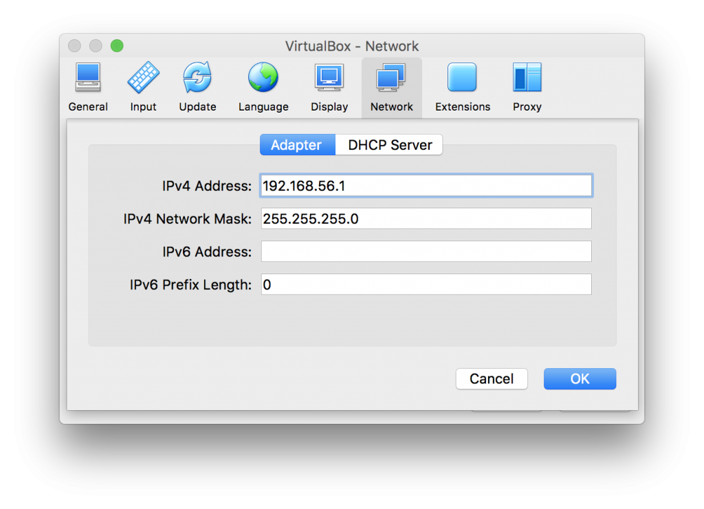
  2. Once installed go to VirtualBox menu and choose “Preferences” and click “Network”.
  3. Click “Host-only Networks” and choose icon add: 
  4. Now you have new “Host-only Network” which is needed for incoming connections. You can check the details by double clicking vboxnet0:
  5. Next create VM with two network adapters:
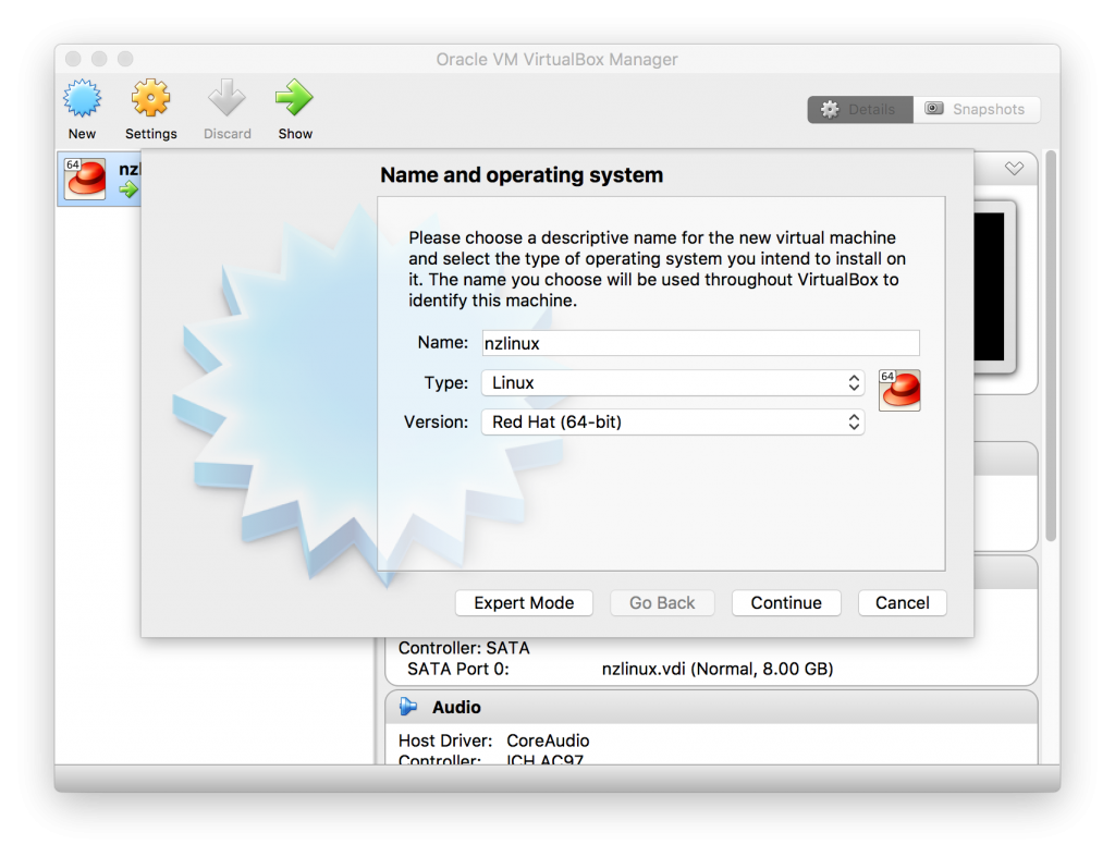
    1. Choose “New” and select “Name”, “Type” and “Version”:
    2. Click continue. You can keep the memory on 1024MB which is the default.
    3. Click continue and choose “Create virtual hard disk now” and click “Create”.
    4.  “Hard disk type” can be VDI, if you do not plan to run VM on other hypervisors, but if you plan to run it on VMWare hypervisor, choose VMDK. Click “Continue”.
    5. For flexibility choose “Dynamically allocated” and for best performance choose “Fixed size”.
    6. For most purposes 8.0GB is enough, but your needs may vary. Choose “Create”.
    7. Now VM is created, but we need to change some of the network settings:
      1. While new VM is highlighted, choose “Settings” and select “Network” tab.
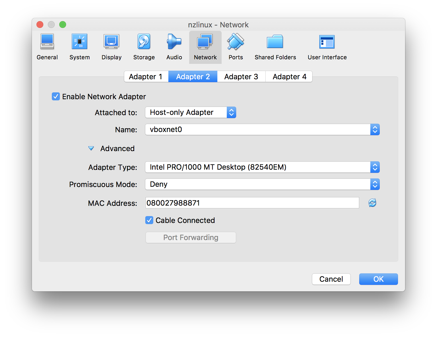
      2. “Adapter 1” default settings are ok for most cases, but we need to add “Adapter 2” so click “Adapter 2”. We need 2nd Network card for incoming connections, so we select “Enable Network Adapter” and set “Attached to: Host-only Adapter”:
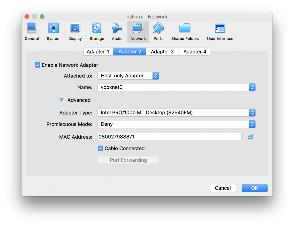
      3. Click “OK”.
  6. We need to have CentOS minimal installation image which we can download from CentOS site: https://www.centos.org/download/
  7. Choose your download site and store the image to desired location. We need it only during intallation.
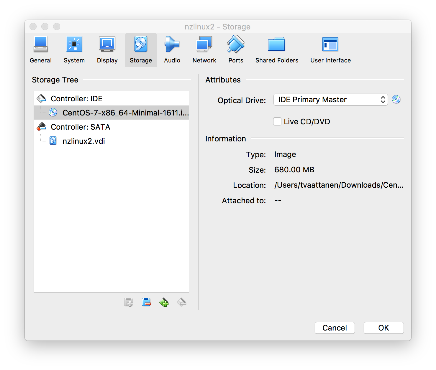
  8. Once downloaded, go back to VM Settings on virtual box:
    1. Select “Storage” tab and “Controller: IDE” and click the CDROM icon and then another CDROM icon on right side from “Optical Drive” selection and “Choose Virtual Optical Disk File”.
    2. Select the CentOS minimal installation disk image you downloaded on previous step:

      1. Click “OK”
  9. Now we can start the CentOS minimal installation. Choose “Install….” when VM has booted.
  10. Next we get graphical installation screen. We can keep language settings as default and click “Continue”:
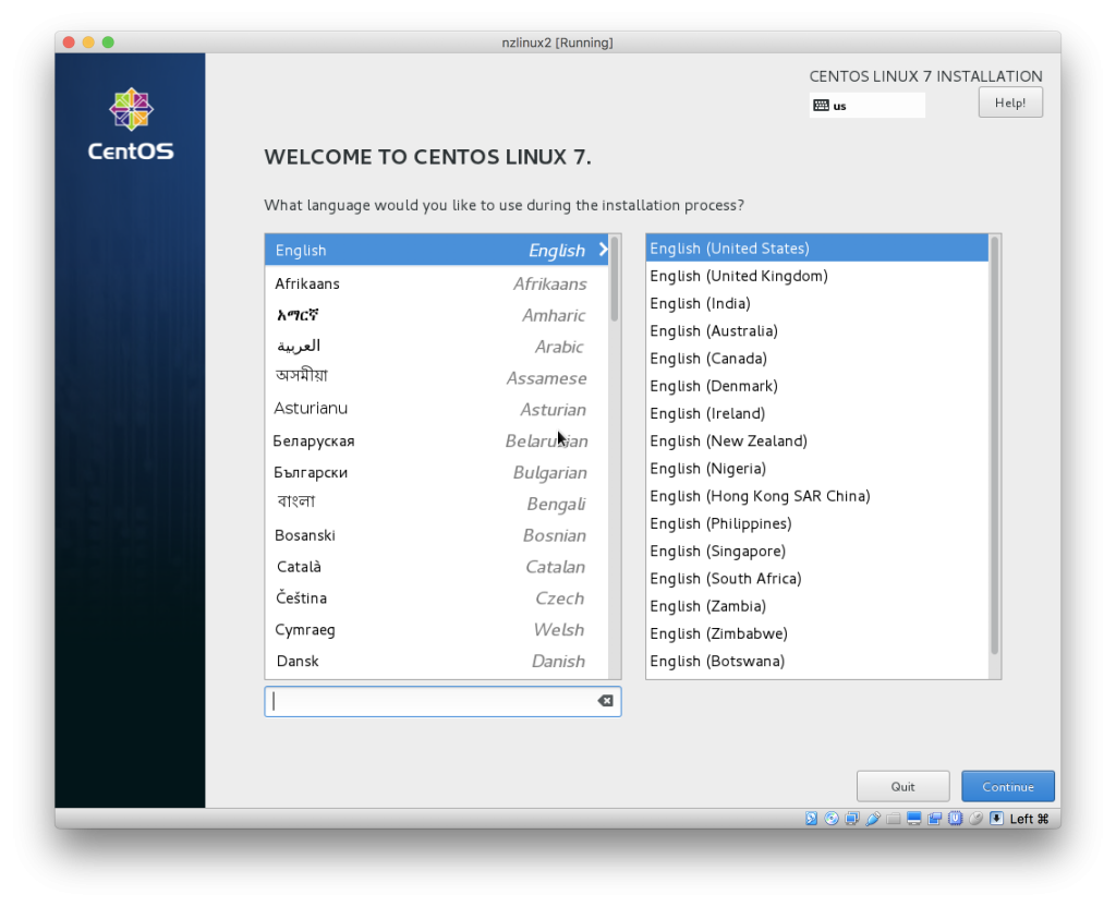
  11. Note when you click the VM, it will grab the mouse. To release the mouse, click left CMD (on MacOS).
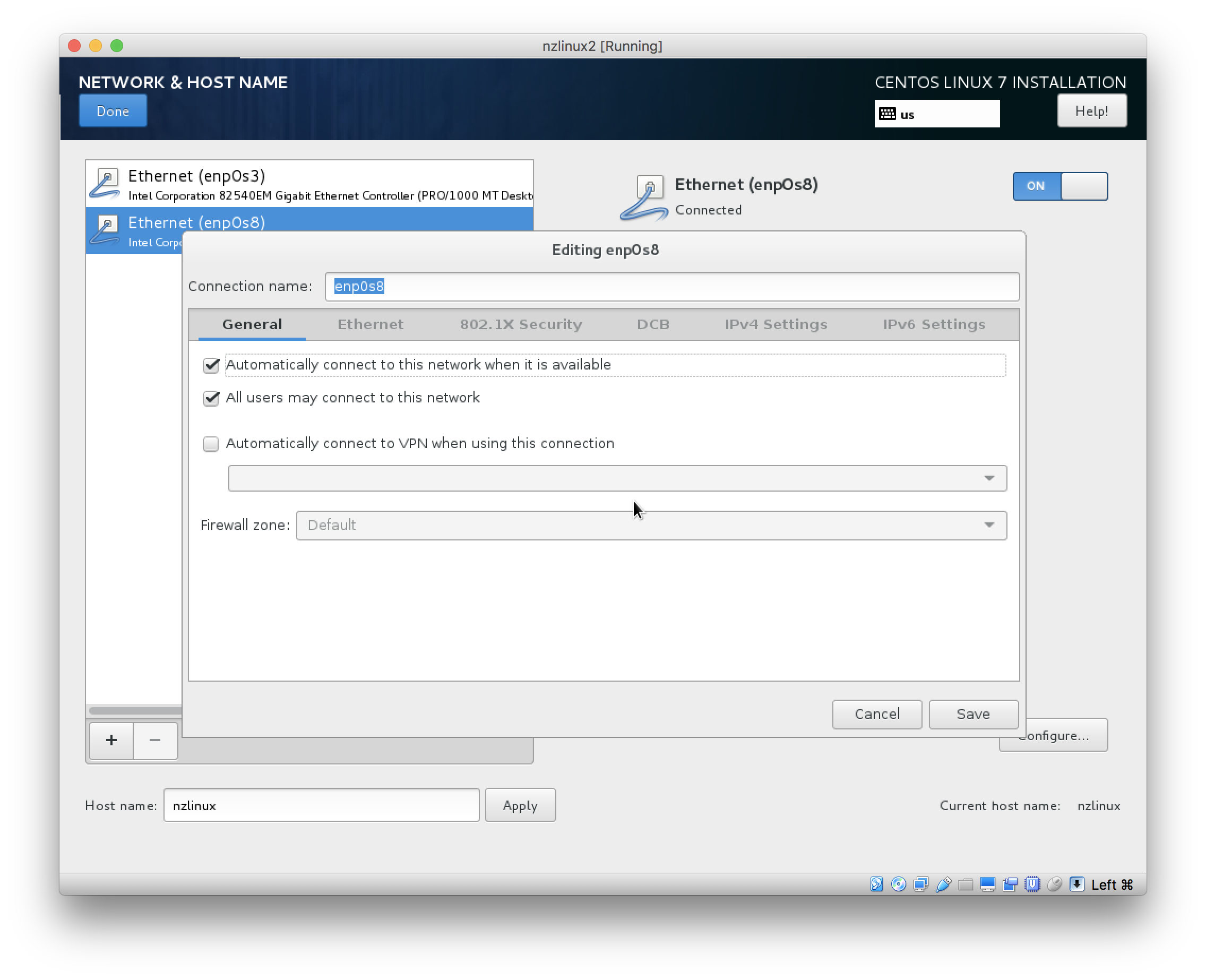
  12. Click “Network & Host name”. You can specify your hostname as preferred.
  13. Both Network cards are off by default. Set them both to “ON”.
  14. For both Network cards, click “Configure” and on “General” tab choose “Automatically connect to this network when it is available”:
  15. Click “Done” to get out from Network settings, and click “Installation Destination” to confirm storage device selected by default is correct (no need to change anything). Then click “Done” to get back to main screen and you can start the installation by selecting “Begin Installation”.
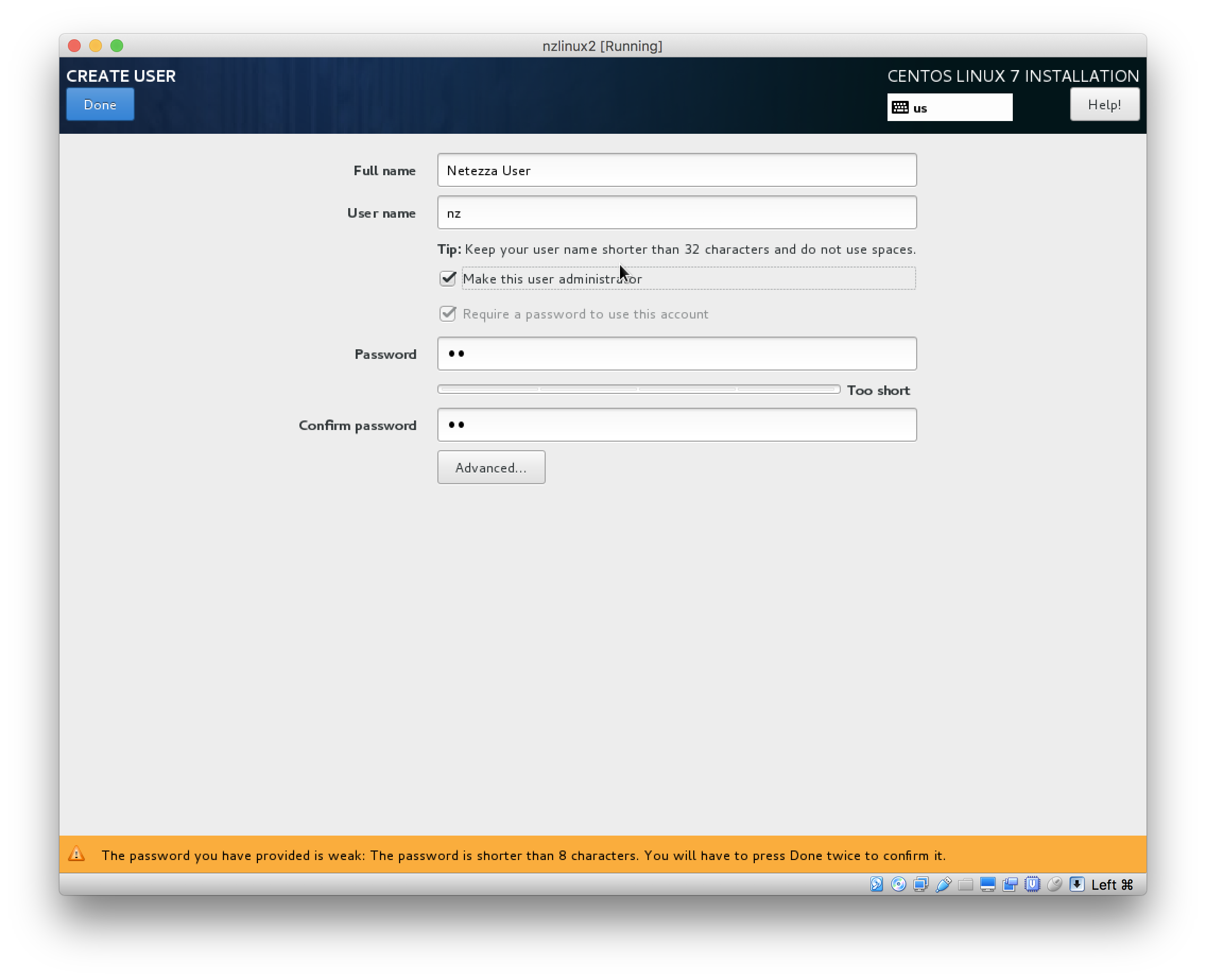
  16. During installation set root password and select to create user. In my examples for setting up Netezza client, I have chosen to create “Netezza User” with username “nz”. I will also make this user an administrator:
  17. Once installation is done you can click “Finnish configuration” and then “Reboot”.
  18. VM boots now first time. You can either ssh to the system (from Terminal on MacOS, or using Putty on Windows).
  19. If this is only VM using Host-only network on VirtualBox, it’s likely the IP is 192.168.56.101. You can check the IP for device enp0S8 with command: ip addr show when logged in through VirtualBox console.
  20. After installation first thing to do is to update all packages with yum update command. Either as root give command “yum -y update” or as administrative user as “sudo yum -y update”.

Configure file sharing between Host and Guest OS

You might want to be able to share, for instance your PycharmProjects folder to run Python code you developed directly on LinuxVM. That is a bit of the whole point for the LinuxVM in this case.

To achieve that, you need to enable file sharing. There is few additional steps needed I’l go through below:

  1. You need few additional packages first. Run following commands as root:
    1. yum -y update
    2. yum -y install gcc kernel-devel make bzip2
    3. reboot
  2. Once LinuxVM has rebooted and you have LinuxVM Window active select from menu “Devices” –> “Insert Guest Additions CD Image…” . Then log in to LinuxVM as root via VirtualBox console or ssh again and run following commands:
    1. mkdir /cdrom
    2. mount /dev/cdrom /cdrom
    3. /cdrom/VBoxLinuxAdditions.run
  3. Now select the folder you want to share from your Host OS to LinuxVM. Go to VM settings and choose “Shared Folders” tab and click icon and then choose the folder you want to share:
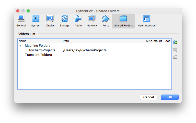
  4. Note: Make sure you set the mount permanent. No need for automount option, since we do it a bit differently below.
  5. Above we are sharing PycharmProjects folder. We want to have PycharmProjects folder mounted on LinuxVM on nz users home directory. As nz user we first create directory PycharmProjects with command: mkdir $HOME/PycharmProjects
  6. Then as root, we add following entry to /etc/fstab:PycharmProjects /home/nz/PycharmProjects vboxsf uid=nz,gid=nz           0 0
  7. After reboot you should now have your PycharProjects folder mounted with read and write access under nz users home directory.

    Note: The purpose for above share is, that when you develop your Python code with Pycharm on MacOS and if your code needs connection to Netezza, you can not run it on MacOS, since there is no Netezza drivers. Instead, when following this guide, you will be able to run you Pycharm edited code seamlessly on the LinuxVM through ssh connection, and once confirmed to work, you can commit your changes.

Install Python 3.6 with pyodbc, pandas and sqlalchemy

Log in to LinuxVM as root and run following commands:

yum -y update
yum -y install git
yum -y install yum-utils
yum -y groupinstall development
yum -y install https://centos7.iuscommunity.org/ius-release.rpm
yum -y install python36u
yum -y install python36u-pip
yum -y install python36u-devel
pip3.6 install pandas
yum -y install unixODBC-devel
pip3.6 install pyodbc
yum -y install gcc-c++
yum -y install python-devel
yum -y install telnet
yum -y install compat-libstdc++-33.i686
yum -y install zlib-1.2.7-17.el7.i686
yum -y install ncurses-libs-5.9-13.20130511.el7.i686
yum -y install libcom_err-1.42.9-9.el7.i686
yum -y install wget
yum -y install net-tools
pip3.6 install sqlalchemy
pip3.6 install psycopg2

Testing pyodbc

Edit the connection string accordingly:

[nz@nzlinux ~]$ python3.6
Python 3.6.2 (default, Jul 18 2017, 22:59:34) 
[GCC 4.8.5 20150623 (Red Hat 4.8.5-11)] on linux
Type "help", "copyright", "credits" or "license" for more information.
>>> import pyodbc
>>> pyodbc.connect(server="nz", database="TEST", dsn="NZSQL", user="admin", PWD="password", autocommit=False)
<pyodbc.Connection object at 0x7f66ef8566b0>

Install Netezza Linux client

First you need to download NPS Linux client from IBM Fix Central

Then, as root run following commands (accept all defaults):

mkdir NPS
cd NPS
tar xvfz ../nz-linuxclient-v7.2.1.4-P2.tar.gz
cd linux
./unpack
cd ../linux64
./unpack

Now, log in as nz user and add following lines to $HOME/.bashrc (modify credentials and server details accordingly: NZ_USER, NZ_PASSWORD and NZ_HOST):

NZ_HOST=netezza.domain.com
NZ_DATABASE=SYSTEM
NZ_USER=admin
NZ_PASSWORD=password
export NZ_HOST NZ_DATABASE NZ_USER NZ_PASSWORD
export LD_LIBRARY_PATH=$LD_LIBRARY_PATH:/usr/local/nz/lib64
export PATH=$PATH:/usr/local/nz/bin
export ODBCINI=$HOME/.odbc.ini
export NZ_ODBC_INI_PATH=$HOME

To make above changes effective without logging out and in, you can instead run command: . ./.bashrc

Now you should be able to use nzsql:

[nz@nzlinux ~]$ nzsql
Welcome to nzsql, the IBM Netezza SQL interactive terminal.
Type:  \h for help with SQL commands
       \? for help on internal slash commands
       \g or terminate with semicolon to execute query
       \q to quit
SYSTEM.ADMIN(ADMIN)=>

Setup ODBC

Copy following two files, odbc.ini and odbcinst.ini to /etc as root:

odbc.ini
odbcinst.ini

As nz user create following symlinks:

ln -s /etc/odbcinst.ini .
ln -s /etc/odbc.ini .
ln -s /etc/odbc.ini .odbc.ini
ln -s /etc/odbcinst.ini .odbcinst.ini

 Questions

If you have any questions, please connect with me.

Update

The .odbc.ini and .odbcinst.ini issues seems to be fixed with newer Python versions, so creating symlinks to users home directory nor creating system files under /etc are not anymore required. Just using .odbc.ini and .odbcinst.ini in user’s home directory works now as it is supposed to work.

How to set up SQuirreL SQL Client for Netezza

This article describes how to set up SQuirreL SQL Client for Netezza. There is not much free SQL query tools available for MacOS and Linux, but SQuirreL is an exception. It uses JDBC for connecting to Netezza, so first thing you need is Netezza JDBC driver. Netezza JDBC driver you can find  for example from latest Netezza Linux client, for example (it is inside npsclient.7.2.1.X-PX.tar.gz  as lib/nzjdbc3.jar).

Download and install SQuirreL SQL Client

  1. Download SQuirreL jar installer package from: http://www.squirrelsql.org/
  2. You need to have Java JDK installed to run and install SQuirreL. As of writing this HOWTO latest JDK can be downloaded from: http://www.oracle.com/technetwork/java/javase/downloads/jdk8-downloads-2133151.html
  3. Once the jar installer is downloaded, run it with: java -jar squirrel-sql-3.7.1-MACOSX-install.jar
  4. Accept the defaults and choose which plugins you need. In my example I have chosen plugins “Multi source”, “Data import”, “MySQL”, “Netezza”, “Oracle”, “PostgreSQL”, “Session Scripts”. “Smart Tools”, “SQL Parametrisation”, “SQL Replace” and “SQL Validator” .
  5. Click Next and Done and you have SQuirreL SQL Client installed on you system.

Configure SQuirreL SQL Client for Netezza

Before beginning configuring the driver, you need to have Netezza JDBC driver nzjdbc3.jar stored on you computer. Netezza JDBC driver can be found for example from Netezza Linux Client under the 32bit Linux tar archive.

Configure the Netezza driver

Once SQuirreL SQL Client is started, first thing to do, is to add Netezza JDBC driver to available drivers on SQuirrelL SQL CLient. In Netezza’s case, there is no Netezza driver on list of drivers, so we will add one.

  1. I stored Netezza JDBC driver under $HOME/Java, but you can choose a different location.
  2. Click Drivers tab and and then click  sign to add new driver.
  3. Highlight “Extra Class Path” tab and click “Add” to add the Netezza JDBC driver you have earlier stored to you computer.
  4. Set “Name” to “Netezza”, “Example URL” to “jdbc:netezza://<host>:5480/<dbname>”, “Websitete URL” to “http://ibm.com” and most importantly set “Class Name” to “org.netezza.Driver”. Once done, click “OK”.

Setup connection to Netezza database

Since SQuirreL SQL Client uses JDBC for connecting to database, it can in theory have only one connection per database. So you need to create one connection per database you are working on because of the JDBC limitation. There is commercial tools like RazorSQL which you can have only one database connection and still connect and query all databases with that same connection, but with SQuirreL SQL Client this is not the case.

  1. To set up your first Netezza database connection on SQuirreL SQL Client, select the “Aliases” tab and click  icon, to add new database connection.
  2. From “Driver pull down list select “Netezza”.
  3. Choose “Name” for you connection ie. the database name you are connecting to.
  4. URL is the form you set up when creating the driver: “jdbc:netezza://<host>:5480/<dbname>”. Set “host” and “dbname” accordingly.
  5. Now you can test the connection. Click “Test” and then “Connect”. If connection is unsuccesful, check the trace to find out the reason.
  6. Once alias is created, you can connect to database. Either double click the alaias or right click it and select connect.

Questions?

If you have any questions or feedback, please connect with me.

Five steps to tune Netezza query performance

Netezza is designed with simplicity in mind. You can get it up and running in hours rather than weeks. When you follow the basic rules, 99 percent of your applications and queries can perform well. There are six things you should keep in mind while designing your databases and setting up maintenance tasks:

  • Distribution
  • Data types
  • Statistics
  • Zone maps
  • Data organization
  • Groom

When you have taken care of the these things, you shouldn’t have any major issues with performance. However, if you do have issues, how do you find them? Follow these five steps, which can help you to find and possibly fix the performance issues on your appliance.

1. Use IBM Netezza Performance Portal and the query history database

The IBM Netezza Performance Portal is an excellent tool for making sure you have everything in place, and if you don’t it will help you to identify any issues. It provides an excellent front end to the query history database and it is able to connect the appliance performance history with your query history.

Netezza Performance Portal and its installation guide are available for download from IBM Fix Central. The installation is fairly simple. Please refer to the “IBM Netezza Performance Portal User’s Guide” (which is included in the download) for installing and configuring both Netezza Performance Portal and the query history database.

2. Check the server load and resources

One of the greatest things about Netezza Performance Portal is its ability to monitor one or more Netezza systems and their resource usage. From the nice graphical user interface (GUI) you can easily identify performance peaks. Then, if you see any changes in trend, you can drill down and take a closer look by using your mouse pointer to click where the change begins and ends. You can repeat this as many times as you want. After zooming in on the period of time you are interested in, you can click the “Jump to History” button to see which queries were running during that time slot. But first you will need to choose the host you are interested in, as this will populate the “Submit Time” and “Finish Time” fields in the query history view.

3. Identify the problematic queries

Identifying problematic queries is, of course, easier said than done. Basically, there are three different types of long-lasting queries that usually require a closer look:

  • Queries that take a long time to finish because they need to access a lot of data.
  • Queries that take long time to finish because the query is not optimal.
  • Queries that take a long time to finish because the database design is not optimal.

When you first look at your queries, they probably just look like long-lasting queries. However, if you know your data and your queries, you might be able to place at least some of them in the first class I mentioned (queries that naturally take a long time to finish because of large amounts of data). What I usually do myself, after I have zoomed in on a performance peak or otherwise interesting period from the Netezza Performance Portal monitoring view, is sort the queries based on their “Query Duration.” I simply list the queries in descending order and then look at the “Query Text.”

When you have selected the interesting query, you can perform various actions with Netezza Performance Portal, including the following:

  • You can right-click the query and check the “Identical Query Trend Chart.” This will give you an idea of the variation in duration for identical queries over time. For instance, if the system is overwhelmed by concurrently running workloads, it is obvious that a query will not run as fast as it normally would. If you notice that a query took longer than normal to run, you should check what else was running on the system at that time.
  • If it really took longer to run than is typical, you can check the “Query/Plan Activity Chart.” This will give you a nice graphical view of all the queries running concurrently on the system, which could be affecting the duration of the query you were interested in.
  • You can check if the statistics are up to date on tables related to the query, and you can even update the statistics thorough Netezza Performance Portal if they are outdated.You can also check encumbrance. There might have been, for instance, loads or aborted ad hoc queries running on the system that negatively affected the system performance. I have once identified the latter to be the case for why highly-prioritized extract, transform and load (ETL) tasks did not finish in time. Since the queries were aborted, they were not seen in the Query/Plan Activity Chart, but rather on the encumbrance view.

Picture 1: Identical Query Trend Chart

4. Check the query plan

You can check the query plan directly from Netezza Performance Portal and that’s not a bad choice. However, what I usually do is check only the plan ID. You can find this from one of the columns when you are listing the queries on the query history view. I then take the plan ID, log in to the appliance and use nz_plan to take a closer look at the query. One advantage of nz_plan is that it lists the interesting snippets early in the file. Another attractive feature is that it rewrites the query very nicely in a readable format.

That said, you can still use the other techniques available to produce the query plan, including the one available directly through Netezza Performance Portal.

Picture 2: Query Plan generated with nz_plan


5. Check the distribution keys and change them if needed

Now that you have the query plan, one of the first things you can check from there are the distribution keys for the tables the query is accessing. Are they what you assumed they were? Are there re-distributions—single or double? If you see something like “1[03]:spu DownloadTableNode distribute into link 2147484337” you know that the table is distributed. If you assumed it isn’t, then you should check the distribution keys again.

Check how it works now when there are no issues

Don’t wait until you have issues. Familiarize yourself on how to monitor performance issues before you have performance issues. If you don’t already have Netezza Performance Portal, install and deploy it. Try and test how nz_plan utility works. Read the query plans. By doing this, you will be ahead of the game and ready to tackle any upcoming issues.

If you have any questions or suggestions related to query performance tuning, please leave a comment. You can also follow me on Twitter @TVaattanen to discuss more about Netezza.

Everything you wanted to know about networking but were afraid to ask (Part Three)

This blog post is the third part of a series about questions you may have wanted to ask about Netezza networking. The first part concentrated on basic Netezza networking, while the second part continued with network bonding and floating IP addresses. This is the third part, which concentrates on advanced configuration options.

Network speed

By default, a Netezza appliance host has two available Peripheral Component Interconnect (PCI) slots for additional PCI cards. Normally you would use one for a 10 GB dual port Network Interface Adapter (NIC) and the second available slot for dual port 8 GB Host Bus Adapters (HBA). The first you could use for 10 GB networking, and the second could be used for Storage Area Networking (SAN) or LAN-Free backups.

Internally, the appliance uses 10 GB networking. Externally, the default is 1 GB. If you want to have 10 GB external networking, then you need to have the additional 10 GB dual port NIC. Assuming you have a 10 GB network infrastructure in place, you most probably want to go directly to 10 GB.

Even if you plan to initially start with 1 GB external networking, you should consider getting the additional 10 GB NIC and 8 GB Host Bus Adapter (HBA), because you are likely going to use them later.

More about network bonding

By default, the appliance has two hosts. Both of the hosts have one external bonded virtual network device, which consists of two physical 1 GB network interfaces. By default, the network bond is created as active/passive, so the maximum bandwidth you can achieve is 1 GB. If you ask, and your network switch supports link aggregation, you can configure the network bond as Active/Active to get a 2 GB link.

As mentioned above, there are two available PCI slots. This means you can also add two 10 GB dual port NICs to those slots. That way, you can bond up to four 10 GB physical network devices together to achieve maximum 40 GB bandwidth.

Another option would be to use two of the 10 GB ports for virtual IP addresses for application connectivity, and the two remaining ones for a backup network. There are plenty of options, when you consider that you can bond together any of the 10 GB ports in any order to create a bonded device, and then you can choose to go for active/active or active/passive mode.

What about LAN-Free?

This section doesn’t actually cover pure TCP/IP networking, but rather connectivity without TCP/IP. As mentioned earlier, you can have 8 GB HBA installed on one or both of the available PCI slots on the hosts. If you decide to have at least one available PCI slot for additional 8 GB HBA, you could use it for LAN-Free backups.

TCP/IP networking is usually done in shared mode, so you have to share the bandwidth with other users—unless you have a dedicated link, which most often you don’t have. With SAN it is easier and more common to create a dedicated link between the appliance and, for example, the backup server. Or you can connect to an external SAN disk through a dedicated link. That of course has clear benefits; when you know exactly how much bandwidth there is and when you don’t need to share it with anyone.

Another benefit with the LAN-Free option is is the CPU usage. TCP/IP implementations tend to have more CPU overhead compared to SAN. I would emphasize the benefit of the dedicated link though, since CPU on the host is rarely limited while dealing with backups, for instance.

Management interfaces

I already mentioned the management IP addresses: usually two per host, one being the host IP itself, and the other being the IP address of the integrated management module (IMM).

The IMM IP addresses are extremely handy if the host itself is not reachable through the host IP due to the fact it has failed with a hardware error, or if there is something wrong with the configuration. Through IMM, you get console access though the web interface, and either debug the problem or fix the configuration issue.

Some clients require a separate management IP, which is not attached to any network devices used by applications and which still has direct TCP/IP connectivity to the host. In this case neither the host IP nor the IMM IP can be used; you need to use some other available physical network port or interface. If this is the case, you should clearly define the requirements, so you can check the available options.

What else?

If anything else is on your mind that you did not dare to ask earlier, feel free to ask or comment below. You can also follow me on Twitter @TVaattanen to discuss more about Netezza.

Everything you wanted to know about Netezza networking but were afraid to ask (Part Two)

This blog post is the second in a three-part series with the goal of answering questions you might have about Netezza networking. The first part concentrates on basic Netezza networking, whereas this second part covers more advanced networking concepts. For advanced configuration options, you can check out the upcoming third part of this blog post.

Network bonding

You have two hosts: active and passive. Each has its own IP address. These IP addresses are not floating. These are called host IPs. Since you want to have maximum redundancy on all components, there are actually two physical network devices virtually bound together to create virtual networking devices (one for each host). Both hosts have two physical network devices that carry one IP address. This is called network bonding.

Let’s say both of the hosts have network devices eth6 and eth7 and they create a coupled virtual device called bond2. We usually use bond0 and bond1 internally, so the first bonded device for external use is normally bond2.

For the virtual device bond2, you can assign an IP address and connect to a host. Both active and passive hosts will have this device and both of the hosts will have their own individual IP address, which is bound to this virtual device.

Virtual IP

If you think of this from an applications point of view, it wouldn’t make sense to connect to the host IP, since if the active host fails, you would need to re-configure applications to use the new active host, which has a different IP.

That’s why applications use virtual IP. Virtual IP is actually an IP alias, which is bound to an active host. Hosts run standard Linux operating systems, so if you are familiar with Linux, it’s easy to explain. If not, it’s still not rocket science. On Linux, you can easily add IP aliases on top of any physical, or virtual for that matter, network device . If you have physical network device eth0 with fictional IP address 192.168.1.100, you can add another IP address to that same physical device just by assigning an IP to device eth0:0. Next you add to device eth0:1 and so on.

In this case, you have virtual network device bond2, which is a bonded device having physical devices eth6 and eth7 behind it. If you lose eth6, you are still good as long as physical device eth7 is good. To connect to either of the hosts directly, you would use the IP address assigned to bond2 on the particular host, or rather the host name you have assigned in your domain name server (DNS) for that IP address.

Floating IP

As I said, applications connect to a virtual IP. The virtual IP is assigned to virtual network device bond2:0. It only exists on an active host. This is something called a floating IP, and it is always on the active host. If Host 1 fails, it will be on Host 2. If, as in my example, device eth6 fails, you have bonded device bond2, which consists of eth6 and eth7, the floating IP is still good on that same appliance as before.

There are two virtualization layers here. One is done though network bonding, the other is done through cluster software. If one of the network devices physically breaks, the network bonding will do the trick, and you are still good to go. If the other appliance breaks, you have clustering software, which can deactivate the bond2:0 on the failing host and create bond2:0 on new active host.

So the bond2:0 always has the virtual IP your applications are able to use. You should, of course, always assign host names in your DNS for this virtual IP, and use this host name in your applications instead of using IP addresses directly. That way, if you ever need to change the IP address for the virtual IP, you don’t need to change configurations for several applications. Instead, you just have to change the IP for the host name you have defined for the virtual IP in your DNS configuration.

What about changes to the default configuration?

I will cover advanced configuration options in part three of this blog post. If you have any network-related questions or suggestions, please add them below in the comments. You can also follow me on Twitter @TVaattanen to discuss more about Netezza.

Everything you wanted to know about Netezza networking but were afraid to ask (Part One)

This blog post is the first of three parts informing you about everything you always wanted to know Netezza networking but were afraid to ask.

Simplicity

PureData System for Analytics is a simple appliance for serious analytics. There is minimal tuning involved and it can be up and running in hours with minimal administration. Since it is so simple, you might be afraid to ask questions such as the following:

  • How would my applications connect to the appliance?
  • How am I going to manage the appliance?
  • What is the network bandwidth?

The answer to all of the above questions is that you can do it through a standard TCP/IP networking interface. Well, how do you network with PureData System for Analytics, then?

Connectivity

It’s simple because it’s an appliance. It has basically one IP address, or host name, that your applications use to connect. To manage the appliance, you can use the same IP address or host name for sure, but let’s be a bit more exact.

The PureData System for Analytics appliance has five external IP addresses and six ethernet drops by default.

The appliance consists of two hosts and several S-Blades or Snippet Processing Units (SPUs). One of the hosts is active and the other is passive. You always connect to the appliance through the active host. On the application level, you never connect through any other component. To connect to the active host you use something called a virtual IP or the Open Database Connectivity (ODBC) host name. That IP or host name is for applications. It is a floating virtual IP address which is always on an active host.

You should always make sure there is a host name assigned to the virtual IP in your name server so that applications can connect through a Fully Qualified Domain Name (FQDN) instead of an IP address.

Management IPs

To manage the appliance, you can connect directly by using the IP addresses assigned to both hosts, which are called the host IPs. These IPs are assigned to virtual network device bond2 by default, which is created from two physical network devices for redundancy. That would be a normal situation.

You have other options as well. With an integrated management module (IMM) that has an IP address, you can connect and get console access through the network instead of needing to be physically near the appliance.

In summary

There are two physical network devices on both hosts, which creates a virtual network device bond2 by default and one physical network device on IMM on both hosts. That makes six ethernet drops.

There are five IP addresses: One IP address for applications, one IP for both of the two hosts and one IP address for IMM on both of the hosts. Here’s a little more detail:

  • One VIP and ODBC host name: You should define the host name in your name server for VIP. That way, applications are able to use a floating IP through the ODBC host name to connect to the appliance. This IP is assigned to active hosts automatically.
  • Two Host IPs: These are by default assigned to virtual device network bond2 on both hosts. If you want to connect to host 2, you use the IP address assigned to device bond2 on host 2.
  • Two IMM IPs: Both hosts have an integrated management module, you can use them to get direct console access through the network.

The rest of the networking

I will cover more advanced networking topics in part two and three of this blog post series. If you have PureData System for Analytics networking related questions in mind you did not dare to ask earlier, please do it below by commenting on this post. You can also follow me on Twitter @TVaattanen to discuss more about Netezza